Parallel Haskell challenge (also, how to make your research project fail)

In September 2012, after playing with Haskell for a couple of months, I decided to go serious with functional programming as a research topic. By that time I came across many papers and presentations about parallel Haskell, all of them saying how great Haskell is for doing parallel and concurrent computations. This looked very interesting, especially that in my PhD thesis I used an algorithm that seemed to be embarrassingly parallel in nature. I wanted to start my research by applying Haskell to something I am already familiar with so I decided to write efficient, parallel Haskell implementation of the algorithm I used in my PhD. This attempt was supposed to be a motivation to learn various approaches to parallel programming in Haskell: Repa, DPH, Accelerate and possibly some others. The task seemed simple and I estimated it should take me about 5 months.

I was wrong and I failed. After about 6 months I abandoned the project. Despite my initial optimism, upon closer examination the algorithm turned out not to be embarrassingly parallel. I could not find a good way of parallelizing it and doing things in functional setting made things even more difficult. I don’t think I will ever get back to this project so I’m putting the code on GitHub. In this post I will give a brief overview of the algorithm, discuss parallelization strategies I came up with and the state of the implementation. I hope that someone will pick it up and solve the problems I was unable to solve. Consider this a challenge problem in parallel programming in Haskell. I think that if solution is found it might be worthy a paper (unless it is something obvious that escaped me). In any case, please let me know if you’re interested in continuing my work.

Lattice structure

The algorithm I wanted to parallelize is called the “lattice structure”. It is used to compute a Discrete Wavelet Transform (DWT) of a signal ((Orthogonal transform, to be more precise. It is possible to construct lattice structures for biorthogonal wavelets, but that is well beyond the scope of this post.)). I will describe how it works but will not go into details of why it works the way it does (if you’re interested in the gory details take a look at this paper).

Let’s begin by defining a two-point base operation:

$$\left\[ \begin{array}{c} x' \\\\ y' \\end{array} \right \] = \left\[ \begin{array}{cc} \cos \alpha & \phantom{-}\sin \alpha \\\\ \sin \alpha & -\cos \alpha \end{array} \right\] \cdot \left\[ \begin{array}{c} x \\\\ y \\end{array} \right \]$$

This operations takes two floating-point values x and y as input and returns two new values x’ and y’ created by performing simple matrix multiplication. In other words:

$$ x' = x \cdot \cos \alpha + y \cdot \sin \alpha \\\\ y' = x \cdot \sin \alpha - y \cdot \cos \alpha $$

where α is a real parameter. Base operation is visualised like this:

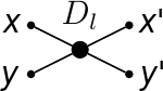
(The idea behind base operation is almost identical as in the butterfly diagram used in Fast Fourier Transforms).

The lattice structure accepts input of even length, sends it through a series of layers and outputs a transformed signal of the same length as input. Lattice structure is organised into layers of base operations connected like this:

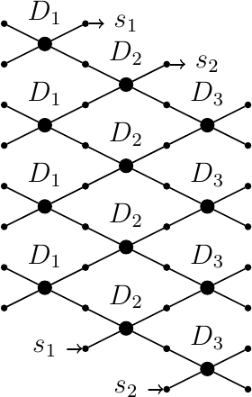
The number of layers may be arbitrary; the number of base operations depends on the length of input signal. Within each layer all base operations are identical, i.e. they share the same value of $latex \\alpha$. Each layer is shifted by one relatively to its preceding layer. At the end of signal there is a cyclic wrap-around, as denoted by latexs_1 and latexs_2 arrows. This has to do with the edge effects. By edge effects I mean the question of what to do at the ends of a signal, where we might have less samples than required to actually perform our signal transformation (because the signal ends and the samples are missing). There are various approaches to this problem. Cyclic wrap-around performed by this structure means that a finite-length signal is in fact treated as it was an infinite, cyclic signal. This approach does not give the best results, but it is very easy to implement. I decided to use it and focus on more important issues.

Note that if we don’t need to keep the original signal the lattice structure could operate in place. This allows for a memory-efficient implementation in languages that have destructive updates. If we want to keep the original signal it is enough that the first layer copies data from old array to a new one. All other layers can operate in place on the new array.

Parallelization opportunities

One look at the lattice structure and you see that it is parallel - base operations within a single layer are independent of each other and can easily be processed in parallel. This approach seems very appropriate for CUDA architecture. But since I am not familiar with GPU programming I decided to begin by exploring parallelism opportunities on a standard CPU.

For CPU computations you can divide input signal into chunks containing many base operations and distribute these chunks to threads running on different cores. Repa library uses this parallelization strategy under the hood. The major problem here is that after each layer has been computed we need to synchronize threads to assemble the result. The question is whether the gains from parallelism are larger than this cost.

After some thought I came up with another parallelization strategy. Instead of synchronizing after each layer I would give each thread its own chunk of signal to propagate through all the layers and then merge the result at the end. This approach requires that each thread is given an input chunk that is slightly larger than the expected output. This results from the fact that here we will not perform cyclic wrap-around but instead we will narrow down the signal. This idea is shown in the image below:

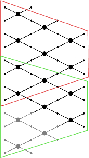
This example assumes dividing the signal between two threads. Each thread receives an input signal of length 8 and produces output of length 4. A couple of issues arise with this approach. As you can see there is some overlap of computations between neighbouring threads, which means we will compute some base operations twice. I derived a formula to estimate amount of duplicate computations with a conclusion that in practice this issue can be completely neglected. Another issue is that the original signal has to be enlarged, because we don’t perform a wrap-around but instead expect the wrapped signal components to be part of the signal (these extra operations are marked in grey colour on the image above). This means that we need to create input vector that is longer than the original one and fill it with appropriate data. We then need to slice that input into chunks, pass each chunk to a separate thread and once all threads are finished we need to assemble the result. Chunking the input signal and assembling the results at the end are extra costs, but they allow us to avoid synchronizing threads between layers. Again, this approach might be implemented with Repa.

A third approach I came up with was a form of nested parallelism: distribute overlapping chunks to separate threads and have each thread compute base operations in parallel, e.g. by using SIMD instructions.

Methodology

My plan was to implement various versions of the above parallelization strategies and compare their performance. When I worked in Matlab I used its profiling capabilities to get precise execution times for my code. So one of the first questions I had to answer was “how do I measure performance of my code in Haskell?” After some googling I quickly came across criterion benchmarking library. Criterion is really convenient to use because it automatically runs the benchmarked function multiple times and performs statistical analysis of the results. It also plots the results in a very accessible form.

While criterion offered me a lot of features I needed, it also raised many questions and issues. One question was whether the forcing of lazily generated benchmark input data distorts the benchmark results. It took me several days to come up with experiments that answered this question. Another issue was that of the reliability of the results. For example I observed that results can differ significantly across runs. This is of course to be expected in a multi-tasking environment. I tried to eliminate the problem by switching my Linux to single-user mode where I could disable all background services. Still, it happened that some results differed significantly across multiple runs, which definitely points out that running benchmarks is not a good way to precisely answer the question “which of the implementations is the most efficient?”. Another observation I made about criterion was that results of benchmarking functions that use FFI depend on their placement in the benchmark suite. I was not able to solve that problem and it undermined my trust in the criterion results. Later during my work I decided to benchmark not only the functions performing the Discrete Wavelet Transform but also all the smaller components that comprise them. Some of the results were impossible for me to interpret in a meaningful way. I ended up not really trusting results from criterion.

Another tool I used for measuring parallel performance was Threadscope. This nifty program visualizes CPU load during program execution as well as garbage collection and some other events like activating threads or putting them to sleep. Threadscope provided me with some insight into what is going on when I run my program. Information from it was very valuable although I couldn’t use it to get the most important information I needed for a multi-threaded code: “how much time does the OS need to start multiple threads and synchronize them later?”.

Implementation

As already mentioned, one of my goals for this project was to learn various parallelization techniques and libraries. This resulted in implementing algorithms described above in a couple of ways. First of all I used three different approaches to handle cyclic wrap-around of the signal between the layers:

cyclic shift - after computing one layer perform a cyclic shift of the intermediate transformed signal. First element of the signal becomes the last, all other elements are shifted by one to the front. This is rather inefficient, especially for lists.
signal extension - instead of doing cyclic shift extend the initial signal and then shorten it after each layer (this approach is required for the second parallelization strategy but it can be used in the first one as well). Constructing the extended signal is time consuming but once lattice structure computations are started the transition between layers becomes much faster for lists. For other data structures, like vectors, it is time consuming because my implementation creates a new, shorter signal and copies data from existing vector to a new one. Since vectors provide constant-time indexing it would be possible to avoid copying by using smarter indexing. I don’t remember why I didn’t implement that.
smart indexing - the most efficient way of implementing cyclic wrap-around is using indexing that shifts the base operations by one on the odd layers. Obviously, to be efficient it requires a data structure that provides constant-time indexing. It requires no copying or any other modification of output data from a layer. Thus it carries no memory and execution overhead.

Now that we know how to implement cyclic wrap-around let’s focus on the actual implementations of the lattice structure. I only implemented the first parallelization strategy, i.e. the one that requires thread synchronization after each layer. I admit I don’t remember the exact reasons why I didn’t implement the signal-chunking strategy. I think I did some preliminary measurements and concluded that overhead of chunking the signal is way to big. Obviously, the strategy that was supposed to use nested parallelizm was also not implemented because it relied on the chunking strategy. So all of the code uses parallelizm within a single layer and synchronizes threads after each layer.

Below is an alphabetic list of what you will find in my source code in the Signal.Wavelet.* modules:

Signal.Wavelet.C1 - I wanted to at least match the performance of C, so I made a sequential implementation in C (see cbits/dwt.c) and linked it into Haskell using FFI bindings. I had serious doubts that the overhead of calling C via FFI might distort the results, but luckily it turned out that it does not - see this post. This implementation uses smart indexing to perform cyclic wrap-around. It also operates in place (except for the first layer, as described earlier).
Signal.Wavelet.Eval1 - this implementation uses lists and the Eval monad. It uses cyclic shift of the input signal between layers. This implementation was not actually a serious effort. I don’t expect anything that operates on lazy lists to have decent performance in numerical computations. Surprisingly though, adding Eval turned out to be a performance killer compared to the sequential implementation on lists. I never investigated why this happens
Signal.Wavelet.Eval2 - same as Eval1, but uses signal extension instead of cyclic shift. Performance is also very poor.
Signal.Wavelet.List1 - sequential implementation on lazy lists with cyclic shift of the signal between the layers. Written as a reference implementation to test other implementations with QuickCheck.
Signal.Wavelet.List2 - same as previous, but uses signal extension. I wrote it because it was only about 10 lines of code.
Signal.Wavelet.Repa1 - parallel and sequential implementation using Repa with cyclic shift between layers. Uses unsafe Repa operations (unsafe = no bounds checking when indexing), forces each layer after it is computed and is as strict as possible.
Signal.Wavelet.Repa2 - same as previous, but uses signal extension.
Signal.Wavelet.Repa3 - this implementation uses internals of the Repa library. To make it run you need to install modified version of Repa that exposes its internal modules. In this implementation I created a new type of Repa array that represents a lattice structure. With this implementation I wanted to see if I can get better performance from Repa if I place the lattice computations inside the array representation. This implementation uses smart indexing.
Signal.Wavelet.Vector1 - this implementation is a Haskell rewrite of the C algorithm that was supposed to be my baseline. It uses mutable vectors and lots of unsafe operations. The code is ugly - it is in fact an imperative algorithm written in a functional language.

In most of the above implementations I tried to write my code in a way that is idiomatic to functional languages. After all this is what the Haskell propaganda advertised - parallelism (almost) for free! The exceptions are Repa3 and Vector1 implementations.

Results

Criterion tests each of the above implementations by feeding it a vector containing 16384 elements and then performing a 6 layer transformation. Each implementation is benchmarked 100 times. Based on these 100 runs criterion computes average runtime, standard deviation, influence of outlying results on the average and a few more things like plotting the results. Below are the benchmarking results on Intel i7 M620 CPU using two cores (click to enlarge):

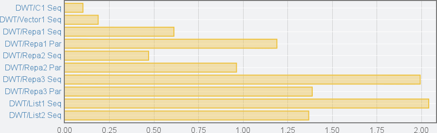
“DWT” prefix of all the benchmarks denotes the forward DWT. There is also the IDWT (inverse DWT) but the results are similar so I elided them. “Seq” suffix denotes sequential implementation, “Par” suffix denotes parallel implementation. As you can see there are no results for the Eval* implementations. The reason is that they are so slow that differences between other implementations become invisible on the bar chart.

The results are interesting. First of all the C implementation is really fast. The only Haskell implementation that comes close to it is Vector1. Too bad the code of Vector1 relies on tons of unsafe operations and isn’t written in functional style at all. All Repa implementations are noticeably slower. The interesting part is that for Repa1 and Repa2 using parallelism slows down the execution time by a factor of 2. For some reason this is not the case for Repa3, where parallelism improves performance. Sadly, Repa3 is as slow as implementation that uses lazy lists.

The detailed results, which I’m not presenting here because there’s a lot of them, raise more questions. For example in one of the benchmarks run on a slower machine most of the running times for the Repa1 implementation were around 3.25ms. But there was one that was only around 1ms. What to make of such a result? Were all the runs, except for this one, slowed down by some background process? Is it some mysterious caching effect? Or is it just some criterion glitch? There were many such questions where I wasn’t able to figure out the answer by looking at the criterion results.

There are more benchmarks in the sources - see the benchmark suite file.

Mistakes and other issues

From a time perspective I can identify several mistakes that I have made that eventually lead to a failure of this project. Firstly, I think that focusing on CPU implementations instead of GPU was wrong. My plan was to quickly deal with the CPU implementations, which I thought I knew how to do, and then figure out how to implement these algorithms on a GPU. However, the CPU implementation turned out to be much slower than I expected and I spent a lot of time trying to actually make my CPU code faster. In the end I never even attempted a GPU implementation.

An important theoretical issue that I should have addressed early in the project is how big input signal do I need to benefit from parallelism. Parallelism based on multiple threads comes with a cost of launching and synchronizing threads. Given that Repa implementations do that for each layer I really pay a lot of extra cost. As you’ve seen my benchmarks use vectors with 16K elements. The problem is that this seems not enough to benefit from parallelism and at the same time it is much more than encountered in typical real-world applications of DWT. So perhaps there is no point in parallelizing the lattice structure, other than using SIMD instructions?

I think the main cause why this project failed is that I did not have sufficient knowledge of parallelism. I’ve read several papers on Repa and DPH and thought that I know enough to implement parallel version of an algorithm I am familiar with. I struggled to understand benchmark results that I got from criterion but in hindsight I think this was not a good approach. The right thing to do was looking at the generated assembly, something that I did not know how to do at that time. I should also have a deeper understanding of hardware and thread handling by the operating system. As a side note, I think this shows that parallelism is not really for free and still requires some arcane knowledge from the programmer. I guess there is a lot to do in the research on parallelism in Haskell.

Summary

I have undertaken a project that seemed like a relatively simple task but it ended up as a failure. This was not the first and probably not the last time in my career - it’s just the way science is. I think the major factor that contributed to failure was me not realizing that I have insufficient knowledge. But I don’t consider my work on this to be a wasted effort. I learned how to use FFI and how to benchmark and test my code. This in turn lead to many posts on this blog.

What remains is an unanswered question: how to implement an efficient, parallel lattice structure in Haskell? I hope thanks to this post and putting my code on Github someone will answer this question.

Acknowledgements

During my work on this project I contacted Ben Lippmeier, author of the Repa library. Ben helped me realize some things that I have missed in my work. That sped up my decision to abandon this project and I thank Ben for that.

UPDATE (18/06/2014), supersedes previous update from (28/05/2014)

One of the comments below suggests it would be interesting to see performance of parallel implementation in C++ or Rust. Thus I have improved the C implementation to use SSE3 SIMD instructions. There’s not too much parallelism there: the main idea is that we can pack both input parameters of the base operation into a single XMM register. This allows to reduce the number of multiplication by two. Also, addition and subtraction are now done by a single instruction. This work is now merged into master. SSE3 support is controlled via -sse3 flag in the cabal file. From the benchmarks it seems that in practice the performance gain is small.

A possible next step I’d like to undertake one day is implementing the lattice structure using AVX instructions. With 256bit registers this will allow to compute two base operations in a single loop iteration. Sadly, at the moment I don’t have access to AVX-enabled CPU.

Back